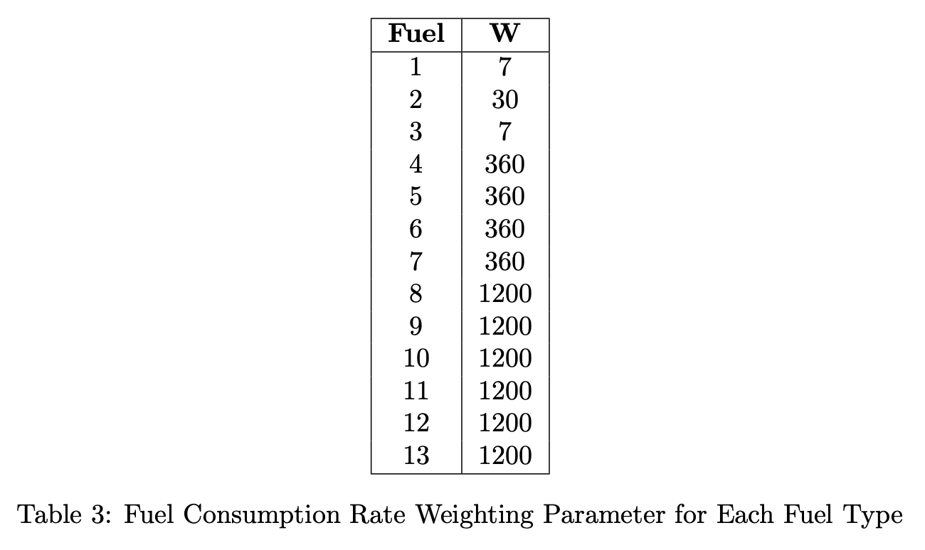
EMBRS Model

EMBRS is a quasi-empirical stochastic cellular automata model. The base of the model is based on the ‘PROPAGATOR’ model. It utilizes a hexagonal grid to discretize regions, the characterstics of each hexagonal cell is based on elevation and fuel data imported from input raster files. The model takes into account the effects of fuel properties, slope, and wind.

Coordinate System

The coordinate system of EMBRS simulations is shown in the diagram below:

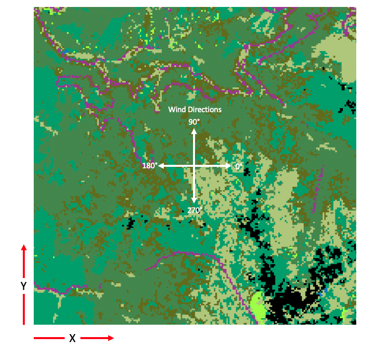
Fig. 2 Coordinate system for EMBRS simulations

Cells

Grid

EMBRS cells are modelled as regular hexagons arranged in a horizontal (pointy topped) grid.

Size

The size of each cell is measured as the distance in meters of each side of a hexagonal cell.

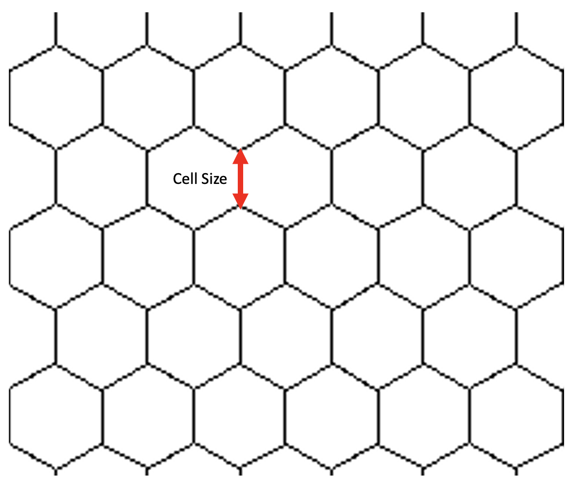
Fig. 3 Hexagon cell size measurement

Elevation

Each cell is assigned an elevation in meters above sea level. The relative elevation between neighboring cells plays a factor in the propagation of the fire.

Fuel

Each cell is assigned one of Anderson’s 13 Fire Behavior Fuel models. Each fuel has different propagation properties that effect the spread of the fire (see Fuels).

Fuel Content

Each cell’s fuel also has a fuel content. This represents the amount of fuel remaining in a cell. If the entire area of a cell contains burnable fuel its fuel content would be 1, meaning 100%. As a cell burns its fuel content decreases as the fuel is burnt (see Fuels: Fuel Consumption Rate).

State

Each cell can be in one of three states at any given time step:

1. Fuel: Cell is not on fire, combustible.

2. Fire: Cell is currently burning.

3. Burnt: Cell was previously on fire, no longer combustible.

The following state transitions can take place:

• Fuel -> Fire:

  • Cell has been ignited by one of its burning neighbors.

• Fire -> Burnt:

  • Cell stops burning because the fuel within it has run out.

• Fire -> Fuel

  • Cell stops burning, but there is fuel remaining (See Prescribed Burns).

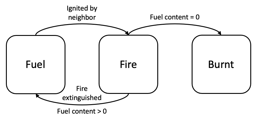
Fig. 4 State transition diagram

Neighborhood

A cell’s neighborhood is defined as the six adjacent cells to it. A cell can only be ignited by one of the cell’s within its neighborhood.

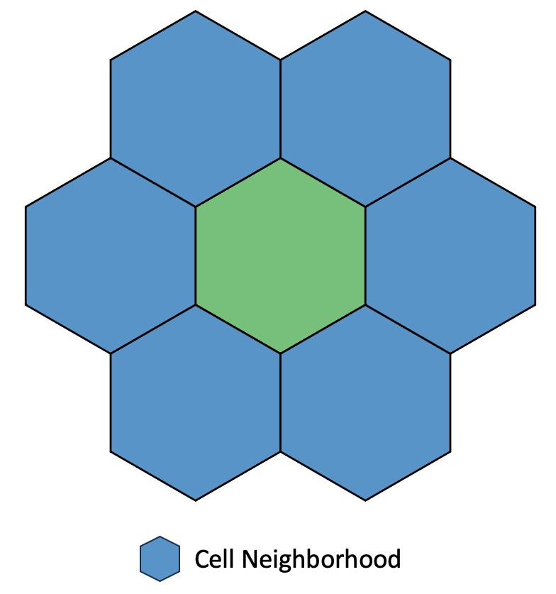
Fig. 5 Hexagonal cell neighborhood

Fuels

EMBRS uses Anderson’s 13 Fire Behavior Fuel models to describe the vegetation in a region. To utilize these fuel types, their properties have been distilled into nominal spread probabilities and nominal spread velocities.

The first 13 fuel models are considered combustible fuel types and can facilitate fire spread while the other five are not combustible.

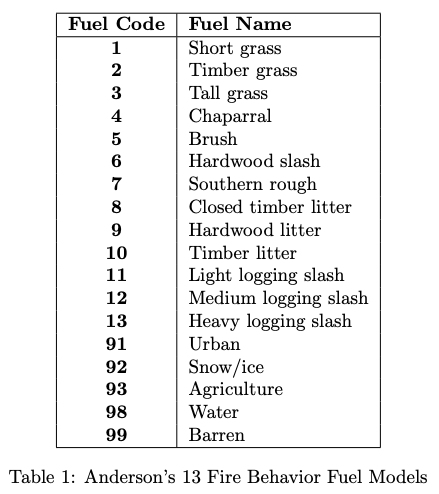
Nominal Spread Probabilities

The nominal spread probability defines a nominal probability that a burning cell of a certain type would ignite a neighboring cell of a certain type. The values are based on the values in PROPAGATOR and have been adjusted based on the properties of each of the FBFMs. These nominal spread probabilities are used as a starting point when calculating the probability of a cell being ignited. More information on this calculation can be found in Ignition Probability. All of the possible combinations’ values are enumerated in the table below:

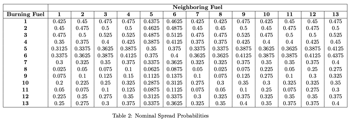
Nominal Spread Velocities

The nominal spread velocity for a fuel is the nominal velocity in ch/hr that a fire would spread within the given fuel type with a 8 km/hr wind as published in Anderson’s paper. These values are used in the ignition probability calculation. The nominal spread velocity for each fuel type is listed in the table below:

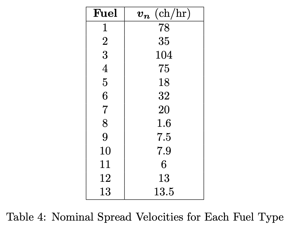
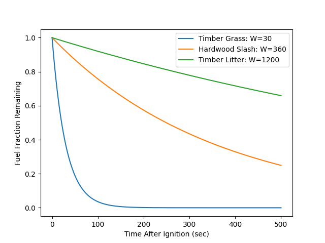
Fuel Consumption Rate

Cells transition from fire to burned once the fuel within the cell is consumed. The rate of fuel consumption is modeled with a semiempirical equation used by (Clark et al. 2004). This models the rate of fuel consumption depending on fuel type. The equation uses a weighting parameter \(W\) which is positively correlated to fuel particle size. The equation can be used to model the remaining fuel content, \(F_c\) at any time \(t\) as follows:

\[F_c(t) = \exp(\frac{-t}{W})\]

The weighting parameters for each fuel type are tabulated below:

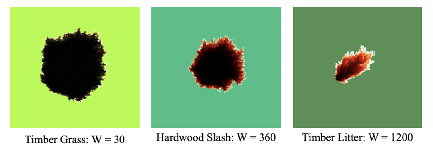
The effect of the weighting parameter can be seen with the mass-loss curves and fire visualizations below:

Fuel Moisture

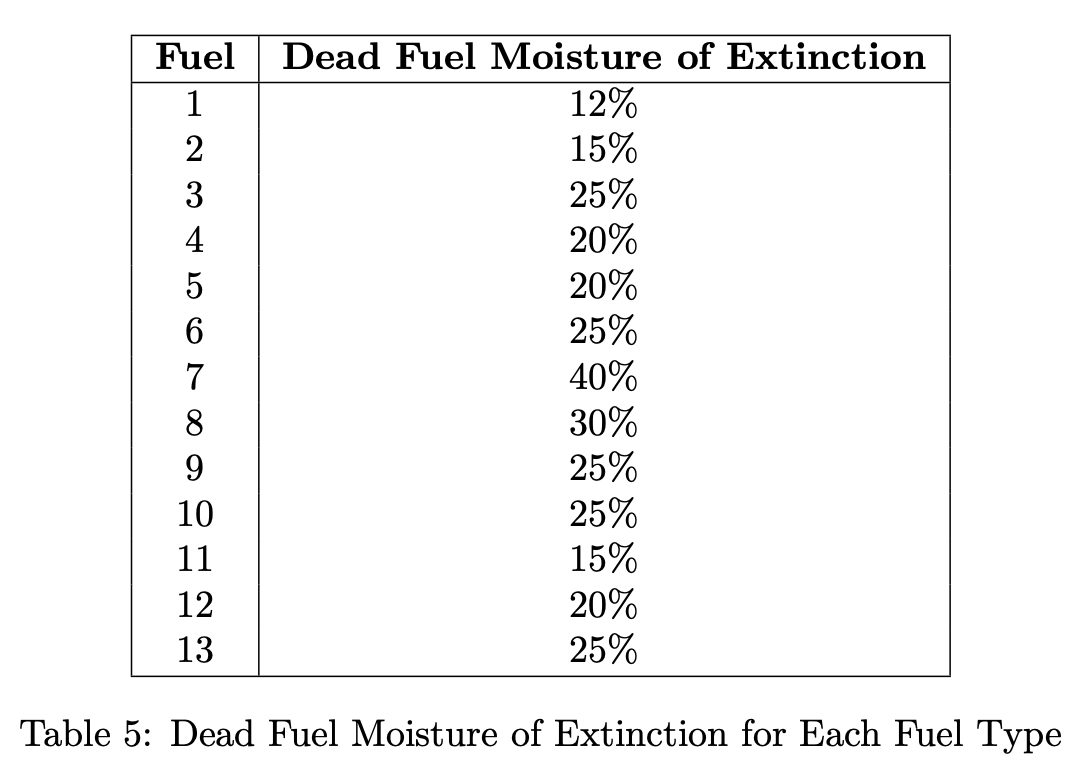
Each fuel in Anderson’s 13 Fire Behavior Fuel Models has a dead moisture of extinction. This is the moisture value where fire will not burn within the given fuel type. These values are listed in the table below:

Each fuel also starts out with a dead moisture content of 8% (standard value in Anderson’s model). If this moisture value increases this will slow down the spread of fire within the cell.

Ignition Probability

Each time-step the ignition probability is calculated for all the unignited neighbors of every burning cell. The calculation is essentially a five-step process:

1. Calculate Wind Effects

To calculate the effects the wind has on the probability we first have to define two vectors:

• Vector \(\mathbf{d}\) represents the displacement between the two cells in question from the burning cell to the un-ignited cell.

• Vector \(\mathbf{w}\) represents the wind vector (units m/s) at the current time-step.

The first wind factor to calculate is \(\alpha_w\). This is combined with the slope factor, \(\alpha_h\) and used in the final probability calculation.

\(\alpha_w\) is defined for different wind speeds based on the below Lorentzian curves:

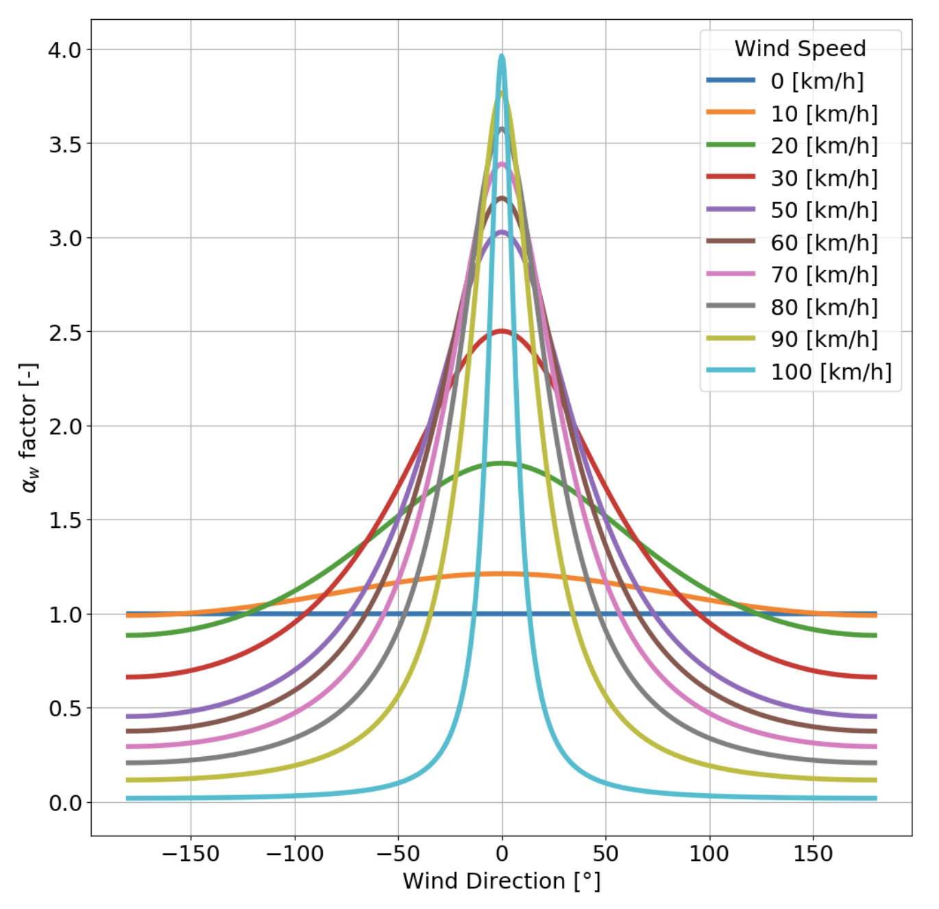
Lorentzian curves are defined by the following equation:

\[L(x) = \frac{A}{x^2 + \gamma^2} + C\]

The parameters defining each wind speed’s curve are tabulated below:

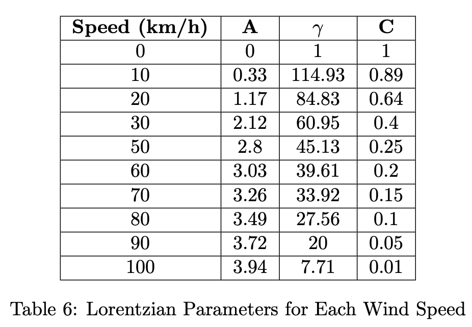
To determine the \(\alpha_w\) equation for intermediate wind speeds, the values above are interpolated to create intermediate Lorenztian curves.

The second wind factor is \(k_w\). This is used to weight the propagation velocity.

\[k_w = \exp\left(0.1783 \times (\mathbf{d} \cdot \mathbf{w})\right) - 0.486\]

2. Calculate Slope Effects

To calculate the effects that slope has on the ignition probability we first need to find the percentage of slope, \(s_{\%}\) and the slope angle, \(\phi\).

Given the vertical positions \(\mathbf{z_c}\) and \(\mathbf{z_n}\) of the current cell and its neighbor respectively, and their x and y positions \(\mathbf{x_c, x_n}\) and \(\mathbf{y_c, y_n}\):

\[ \begin{align}\begin{aligned}\begin{split}s_{\%} & = \left(\frac{z_n - z_c}{\sqrt{(x_c - x_n)^2 + (y_c - y_n)^2}}\right) \times 100 \\\end{split}\\ \phi = \arctan\left(\frac{z_n - z_c}{\sqrt{(x_c - x_n)^2 + (y_c - y_n)^2}}\right)\end{aligned}\end{align} \]

The first slope factor is \(\mathbf{\alpha_h}\). This is combined with \(\mathbf{\alpha_w}\) and used in the final calculation.

\[\begin{split} \alpha_h = \begin{cases} \left( \frac{0.5}{1 + \exp(-0.2 (s_{\%} + 40))} \right) + 0.5 & \text{if } s_{\%} < 0 \\ \left( \frac{0.5}{1 + \exp(-0.2 (s_{\%} - 40))} \right) + 1 & \text{if }s_{\%} \geq 0 \\ \end{cases}\end{split}\]

The second slope factor is \(\mathbf{k_{\phi}}\) this is used to weight the propagation velocity.

\[ \begin{align}\begin{aligned}\begin{split}A = \begin{cases} 0 & \text{if } \phi \geq 0 \\ 1 & \text{otherwise} \end{cases}\end{split}\\ k_\phi = \exp\left(((-1)^A) \times 3.533 \times \tan(\phi)^{1.2}\right)\end{aligned}\end{align} \]

3. Calculate Moisture Effect

There is only one effect from the fuel moisture, \(e_m\). This factor is used in the final calculation of ignition probability.

Given the dead fuel moisture ( m_d ) and the fuel’s dead moisture of extinction \(m_{d_{\text{ext}}}\), we first calculate the ratio:

\[ f_m = \frac{m_d}{m_{d_{\text{ext}}}} \]

Then, \(f_m\) is clipped to not exceed 1:

\[ f_m = \min(f_m, 1) \]

Finally, \(e_m\) is determined as:

\[ e_m = -4.5 \times (f_m - 0.5)^3 + 0.5625 \]

4. Calculate Propagation Velocity

With the effects of the wind and slope calculated, finding the propagation velocity \(v_\text{prop}\) from the nominal propagation velocity, \(v_n\), is straightforward:

\[ v_\text{prop} = v_n \times k_w \times k_\phi \]

Letting \(s\) be the cell size in meters, we can determine the predicted time \(\Delta t\) it will take for the fire to propagate to the neighbor cell as:

\[ \Delta t = \frac{s}{v_{\text{prop}} \cdot f_m} \]

Now, given the simulation time step, \(\delta t\), the predicted number of iterations required for the fire to spread to the neighbor is:

\[ n = \frac{\Delta t}{\delta t} \]

5. Calculate Ignition Probability

Now, combine the wind and slope effects \({\alpha}_{w}\) and \({\alpha}_{w}\).

\[ {\alpha}_{wh} = {\alpha}_{w} \times {\alpha}_{h} \]

Finally, given that \(n_{fc}\) is the fuel contents (between 0-1) of the neighboring cell and using the nominal spread probability, \(p_n\), the ignition probability can be determined:

\[ p_{0} = (1-(1-p_n)^{{\alpha}_{wh}}) \cdot e_m \]

\[p_{ij} = 1 - (1 - p_{0})^\frac{1}{n} \cdot n_{fc}\]

After this value is calculated a random number between 0 and 1 is generated. If that value is less than \(p_{ij}\) the neighboring cell is ignited.

Roads

OpenStreetMap Classifications

Roads can be imported to a map from the OpenStreetMap database (see Creating a Map). OpenStreet map classifies roads into eight classifications, of these eight classifications the following seven are used by EMBRS:

• Motorway

• Trunk

• Primary

• Secondary

• Tertiary

• Residential

• Unclassified

These roads are listed above in decreasing order of how major/trafficked the road is.

Modelling

In wildfire scenarios roads can act as useful anchor points where fire is unlikely to cross or is easier to control. To model this phenomenom in EMBRS, roads are modeled simply as fuel areas with lower fuel contents. The fuel content of a cell that lies on a road depends on the classification of the road in that area. Below is a table of values mapping to road classification to the fuel content along the roads.

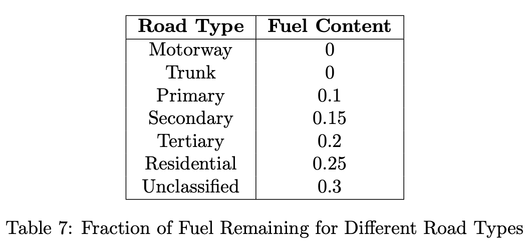
Therefore, the ignition probability calculation is the same for roads, however the reduced fuel content will make an ignition much less likely than in a cell that has 100% of its fuel.

Fire-breaks

Users have the option to specify fire-breaks in a map when creating a map (see Creating a Map). These are regions where the fuel has been reduced by methods such as dozing.

Modelling

When users specify fire-breaks they also specify the percentage of fuel remaining along the break. When modelling these fire-breaks the cells along the fire-break are modified to contain the specified fuel amount. The actual modelling of fire spread does not change from the calculation previously outlined (see Ignition Probability), but the reduced fuel will make fire spread across a fire-break less likely.

Prescribed Burns

In some wildfire fighting scenarios prescribed burns may be carried out to reduce the fuel in large regions in hopes to slow fire spread in that region when the wildfire reaches the area undergoing the prescribed burn. For this reason, one of the available operations that custom control code can carry out is starting a prescribed burn. These fires are modelled much like wildfires with some key differences.

Modelling Differences

Prescribed burns are modeled less intense fires than a wildfire, the following differences in their modelling attempt to reflect that:

Propagation Velocity

The first major difference between prescribed burns and wildfires is their propagation velocity. If a cell is ignited with a prescribed burn the nominal propagation velocity is set as half the value listed in the nominal propagation velocity table above. This reduces the rate at which prescribed burns spread in comparison to wildfires.

Fuel Consumption

The next major difference between prescribed burns and wildfires is the rate at which they consume fuel within the cells they burn. The weighting parameter \(W\) controlling the fuel consumption rate is increased by 50% thus slowing the rate of fuel consumption. Additionally, instead of transitioning to burned when 1% of the overall fuel in the cell remains, prescribed burns will burn only until the fuel within the cell has been reduced by 70% from the fuel content when the burn began.

Wildfire-Prescribed Fire Interaction

In the case where a wildfire and a prescribed fire neighbor one another, a cell containing a wildfire is able to ignite a cell that is on fire due to a prescribed burn. This means the cell that is ignited will now contain a wildfire, not a prescribed fire. The opposite is not true, a cell containing a prescribed fire cannot ignite a cell containing a wildfire.

Note

The above parameters are fully adjustable based on user preferences in ‘utilities/fire_util.py’.